Introduction
2D object detection has for some time been quite successful put simply it can tell where in the image an object sits, which has many use cases. However to place an object in physical dimensions 3D object detection is needed. The figure below shows the natural extension.
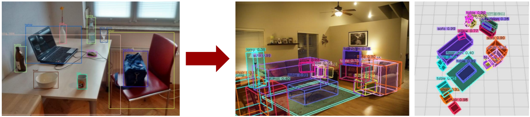
Why 3D object detection is more useful. The squares in the rightmost figure are 1mx1m in size.
Data annotation is difficult
However, one of the biggest challenges with 3D object detection is that large datasets are not widely available. This figure quite nicely illustrates one the reasons why that is - the data rougly takes 11x more time to annotate, and that is not counting how much more difficult it is to collect the data. Collection typically requires complicated setups with depth sensing cameras or whole room scanning.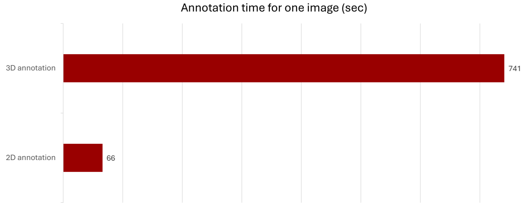
Annotation time motivation.
This begs the question: How to make a 3D object detection model using only 2D annotation boxes
So we’re not interested in making the best possible 3D object detector, but one that is efficient with its use of data. That is why we call it weakly supervised 3D object detection.
The problem is more difficult
This project only concerns using a single camera, so-called monocular object detection. This makes this model much more accessible, as anyone with a simple camera for example a phone can use the model to generate predictions. An issue with this problem is that it makes the problem much more difficult, to determine the physical location of an object one requires at least 2 distinct view points. Without this, you have to resort to estimation.
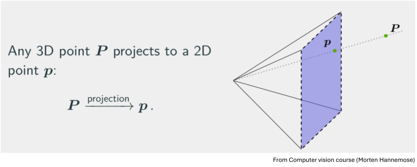
A point in an image, corresponds to an infinite number of points in 3D.
The figure shows how estimating the depth is the biggest challenge, because a large object far away visually appears the same size as a smaller object close by.
Approach: “Weak Cube R-CNN”
We take heavy inspiration from another model Cube R-CNN, but remove all the components related to its 3D detection capability. As such what remains is essentially a Faster R-CNN model. Our model predicts 3D bounding boxes from the 2D predicted bounding boxes.
The crucial component is how to introduce depth sensing, since we do not have the 3D annotations anymore. To this end we use a depth estimation “Depth Anything” model tuned for metric depth estimation (estimating depth in meters), with this model you can effectively get a pseudo ground truth of the depth of the scene. The figure below shows how this might look for an image.
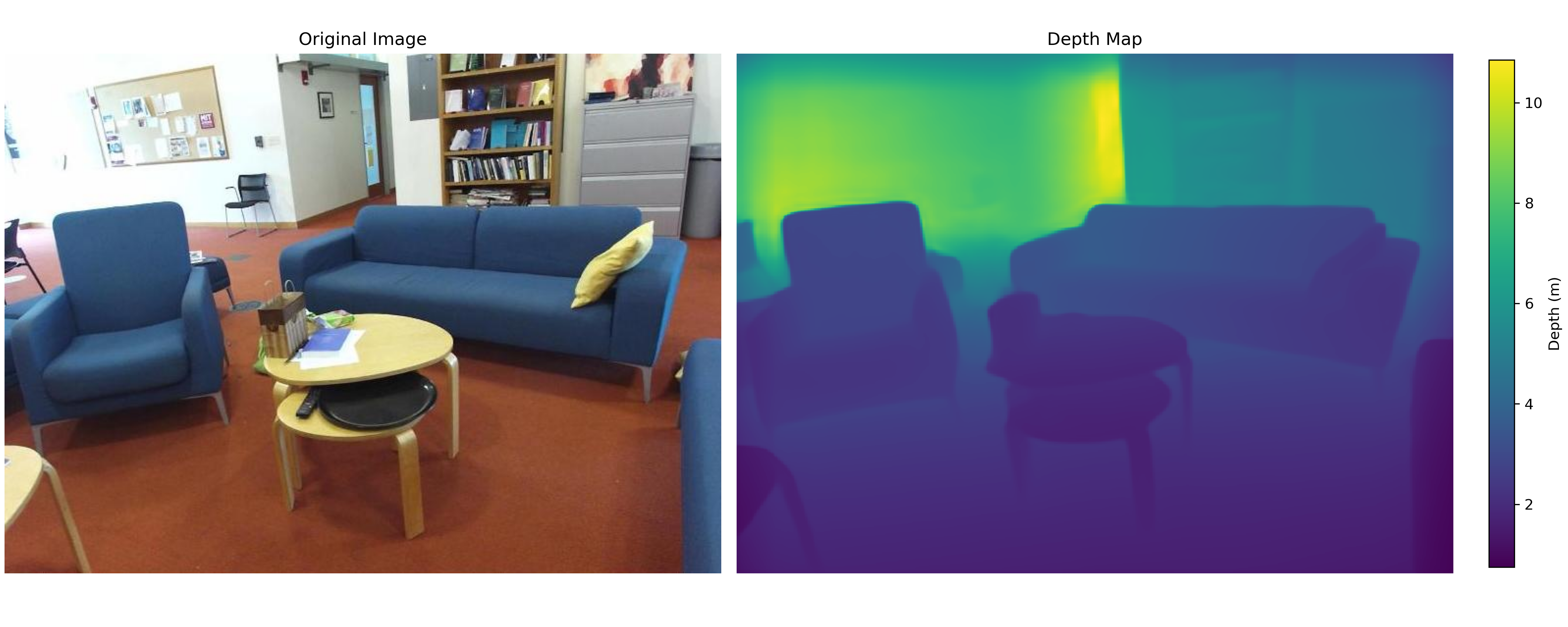
Depth map.
Interestingly, one can also interpret the depth map as a point-cloud by transforming it with simple math. This proves quite useful, because one can use it for other downstream tasks.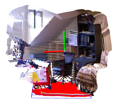
Point cloud generated from a depth map.
When you have the point-cloud it is possible to estimate the ground plane. This is useful because the rotation, along with the depth, is one of the most important characteristics of getting high accuracy. Additionally, it utilises the frame of reference that is present in scenes. However, running a ground estimation algorithm on the point cloud directly is highly unstable, as there are typically other more dominant planes in a scene, like the walls. We overcome this by using a combination of the GroundingDINO and Segment Anything methods (middle image), this effectively filters the ground. Now you can run a simple plane-estimation RANSAC algorithm on the filtered point cloud, this turns out to be quite robust.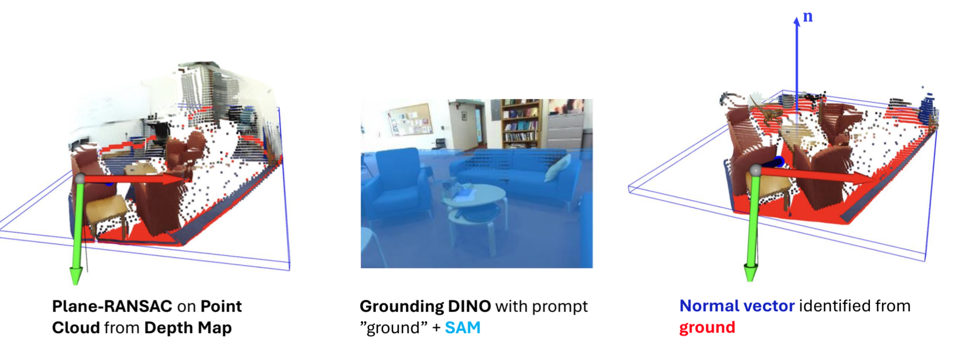
How you can obtain a ground normal from the estimated point cloud.
Based on all of these properties obtained from the scene, we build a variety of loss functions to optimise the model. A large overview of the whole model is shown.
Overview of the whole model
In total the whole optimisation objective for the 3D part of the model becomes: $$ L_{3D} = L_{GIoU} + L_z + L_{dim} + L_{range} + L_{normal} + L_{pose} $$
So we have something for the positioning (first 2), the dimension (middle 2), and the rotation (last 2). These losses are clearly the most important part of the model. Additionally, each term is regularised by a $\lambda$.
Results
For reference to our method we also intially developed a “proposal method” based on the idea of proposing many cubes and selecting the best ones. The ideas generated when developing this method were carried over to our learnable Weak Cube R-CNN method.
Metrics
The notable thing to report on the developed method, is that it achieves higher accuracy than a corresponding fully supervised but annotation time-equalised model.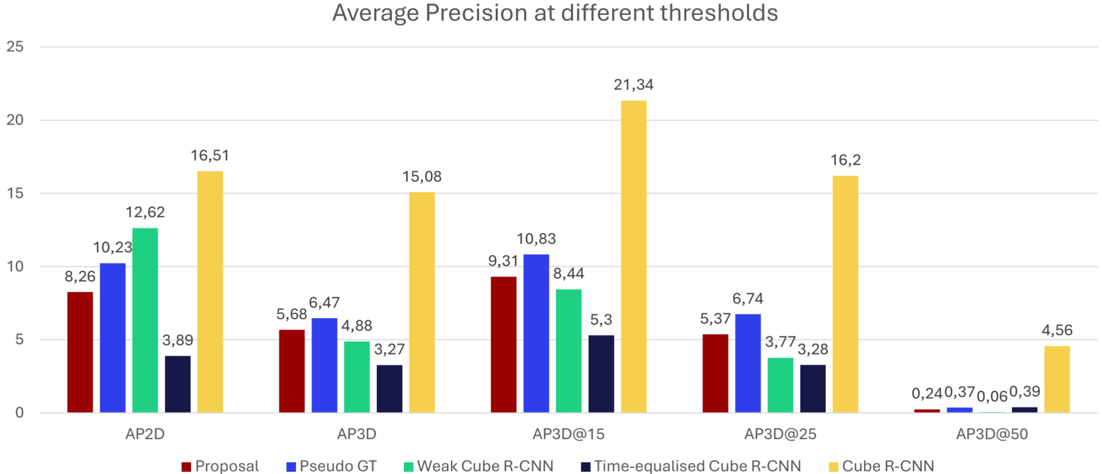
Results on the chosen metric Average precision 2D and 3D
The AP numbers might not look that impressive, but the following figure puts them into context. The AP3D metric is very punishing when just slightly off.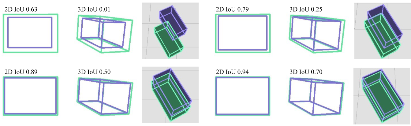
Achieving a high 3D IoU is really hard.
Pictures
What we are here for!!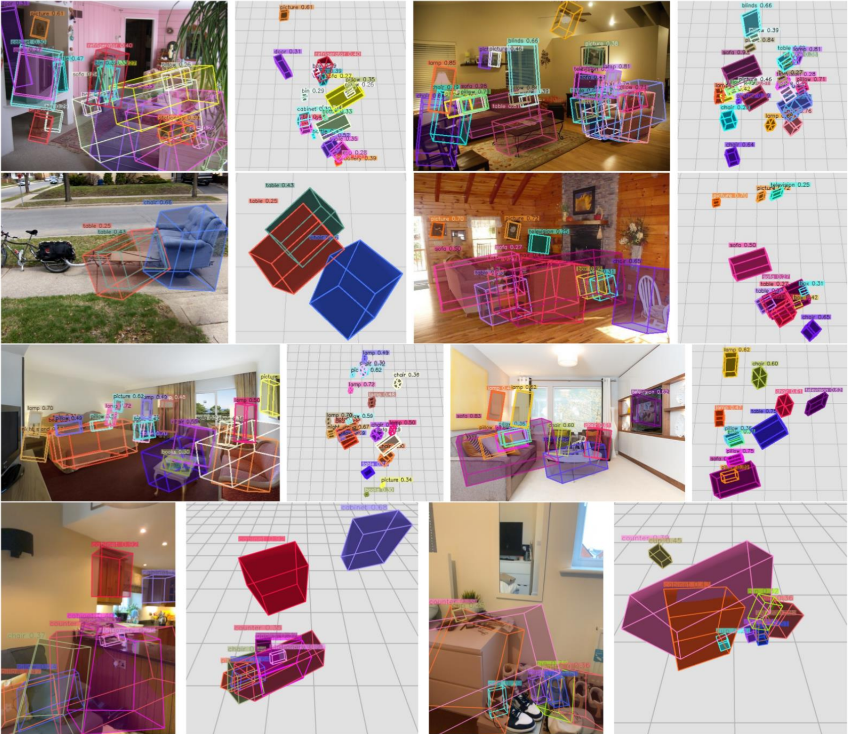
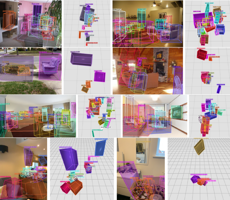
Results from the Weak-Cube R-CNN method
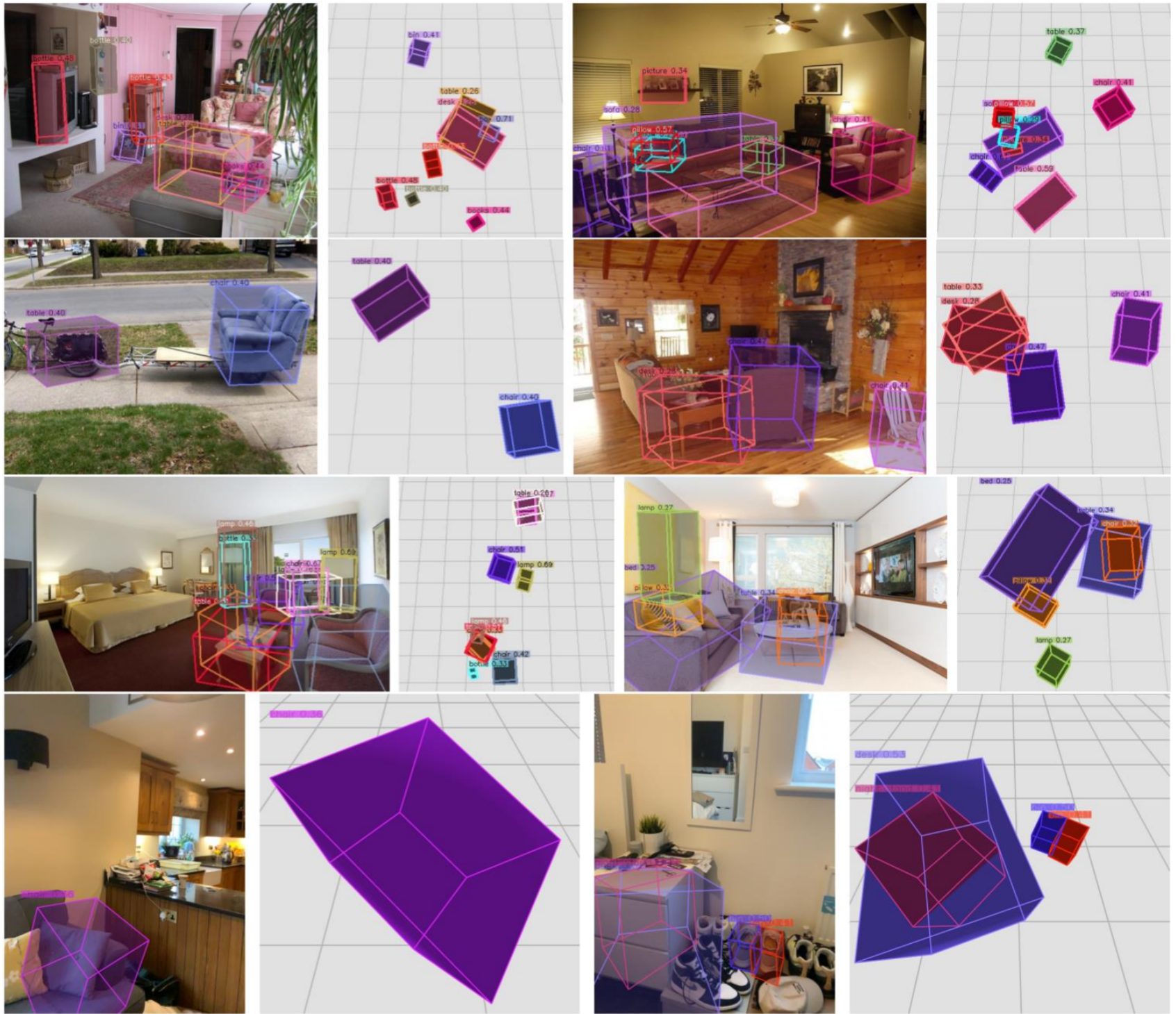
Results from the Annotation time equalised Cube R-CNN method

Results from the standard Cube R-CNN method
Breaking the model
Just trying random stuff, that is really out of domain for the model to see what happens.
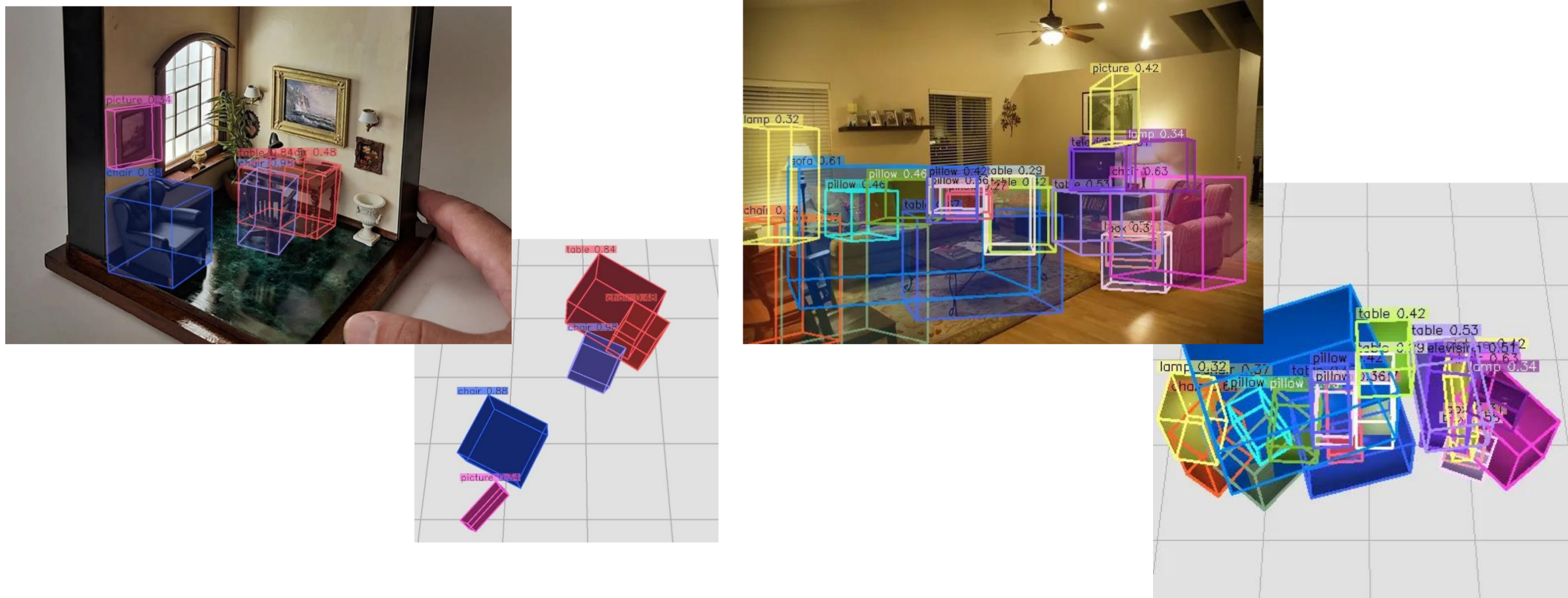
Left: The model predicting wrongly on illusions. Right: When you provide a fake depth map of the same depth, it still looks correct from the front
Huggingface demo
If you want to try the model yourself, we are hosting a demo version on Huggingface.